Plotting Precipitation as Time Series
Now, we will test how different ICON files can be combined together. This is done with 2d_cloud files and a total (domain-average) precipitation time series will be plotted at the end.
Load Python Libraries
[1]:
%matplotlib inline

# system libs
import os, sys, glob
import datetime

# array operators and netcdf datasets
import numpy as np
import xarray as xr
xr.set_options(keep_attrs=True)

# plotting
import pylab as plt
import seaborn as sns
sns.set_context('talk')

import matplotlib.dates as mdates
myFmt = mdates.DateFormatter('%H:%M')
Open Data with xarray
General Paths
[2]:
exercise_path = '/work/bb1224/2023_MS-COURSE'
data_path = f'{exercise_path}/data'
icon_data_path = f'{data_path}/icon-lem'
This is very similar to the tasks already done.
[3]:
os.listdir(icon_data_path)
[3]:
['grids-extpar', 'experiments', 'bc-init']
Now, we select the experimentfolder in which pre-calculated experiments are stored. Later, you need to change this directory to your ICON output directory!
[4]:
exp_name = 'icon_lam_1dom_lpz-base'
exp_path = f'{icon_data_path}/experiments/{exp_name}'
Base Files
[5]:
dset = xr.open_mfdataset( f'{exp_path}/2d_cloud_DOM01_ML_20210516T*Z.nc', chunks={'time':1}, combine='by_coords' )
This is the content of the dataset.
[6]:
dset
[6]:
<xarray.Dataset>
Dimensions:        (time: 288, plev: 1, bnds: 2, plev_2: 1, plev_3: 1,
                    ncells: 10212)
Coordinates:
  * time           (time) float64 2.021e+07 2.021e+07 ... 2.021e+07 2.021e+07
  * plev           (plev) float64 0.0
  * plev_2         (plev_2) float64 400.0
  * plev_3         (plev_3) float64 800.0
Dimensions without coordinates: bnds, ncells
Data variables: (12/17)
    plev_bnds      (time, plev, bnds) float64 dask.array<chunksize=(12, 1, 2), meta=np.ndarray>
    plev_2_bnds    (time, plev_2, bnds) float64 dask.array<chunksize=(12, 1, 2), meta=np.ndarray>
    plev_3_bnds    (time, plev_3, bnds) float64 dask.array<chunksize=(12, 1, 2), meta=np.ndarray>
    tqv_dia        (time, ncells) float32 dask.array<chunksize=(1, 10212), meta=np.ndarray>
    tqc_dia        (time, ncells) float32 dask.array<chunksize=(1, 10212), meta=np.ndarray>
    tqi_dia        (time, ncells) float32 dask.array<chunksize=(1, 10212), meta=np.ndarray>
    ...             ...
    cape           (time, ncells) float32 dask.array<chunksize=(1, 10212), meta=np.ndarray>
    cape_ml        (time, ncells) float32 dask.array<chunksize=(1, 10212), meta=np.ndarray>
    cin_ml         (time, ncells) float32 dask.array<chunksize=(1, 10212), meta=np.ndarray>
    rain_con_rate  (time, ncells) float32 dask.array<chunksize=(1, 10212), meta=np.ndarray>
    prec_con       (time, ncells) float32 dask.array<chunksize=(1, 10212), meta=np.ndarray>
    prec_gsp       (time, ncells) float32 dask.array<chunksize=(1, 10212), meta=np.ndarray>
Attributes:
    CDI:                  Climate Data Interface version 1.8.4 (http://mpimet...
    Conventions:          CF-1.6
    number_of_grid_used:  99
    uuidOfHGrid:          718d4bb6-2c67-4c84-a5ab-440d28412a00
    institution:          Max Planck Institute for Meteorology/Deutscher Wett...
    title:                ICON simulation
    source:               @
    history:              /home/k/k206107/workspace/icon-build/bin/icon at 20...
    references:           see MPIM/DWD publications
comment: v107 Workshop (k206107) on l30004 (Linux 4.18.0-348...Now, the time dimension has a length of 288, i.e. a full day with output each 5 minutes is accumulated. The full data are not loaded into memory so far. We use the capabilities of the dask module to make out-of-memory computations … very convenient!
Adding Grid-Scale and Sub-Gridscale Rain
[7]:
rain = dset['rain_con_rate'] + dset['rain_gsp_rate']
rain.attrs['long_name'] = 'rain rate'
TODO for later: * Is it OK to neglect graupel / snow & hail?
Calculate Average Time Series
[8]:
rain_mean = rain.mean( 'ncells' )
This is still out-of-memory… But, now we do the calculations!
[9]:
rain_mean = rain_mean.compute()
Plot the Time Series
Simple (naive) Plotting
Plotting is now not complicated. We just use the capabilities of xarray.
[10]:
fig = plt.figure( figsize = (14,6))
rain_mean.plot( lw = 3 )
sns.despine()
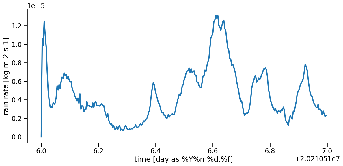
Do you understand this figure? Hmm, time series plotting is perhaps not so simple…
We need to do two things: * convert the rain unit into mm per day * get an understandable time axis.
Unit Conversion
OK, we see the unit kg m-2 s-1. A day has 3600*24 seconds. One liter of water weighs one kilogram. This liter of water put on one square meter has a column height of 1 mm. OK, so far?
[11]:
conversion_factor = 3600 * 24
[12]:
rain_mean = conversion_factor * rain_mean
rain_mean.attrs['units'] = 'mm day-1'
Time Axis
[13]:
rain_mean.time
[13]:
<xarray.DataArray 'time' (time: 288)>
array([20210516.      , 20210516.003472, 20210516.006944, ..., 20210516.989583,
       20210516.993056, 20210516.996528])
Coordinates:
* time (time) float64 2.021e+07 2.021e+07 ... 2.021e+07 2.021e+07
Attributes:
standard_name: time
calendar: proleptic_gregorian
axis: T
units: day as %Y%m%d.%fThe time format is special: %Y%m%d.%f. We use the datetime module to convert the time vector. We will use two function.
[14]:
def convert_time(t, roundTo = 60.):

    '''
    Utility converts between two time formats A->B or B->A:

    Parameters
    ----------
    t : float or datetime object
        time
        A = either float as %Y%m%d.%f where %f is fraction of the day
        B = datetime object
    Returns
    -------
    tout : datetime object or float
        time, counterpart to t
    '''

    t0 = datetime.datetime(1970, 1, 1)

    if type(t) == type(t0):

        tout = np.int( t.strftime('%Y%m%d') )
        date = datetime.datetime.strptime(str(tout), '%Y%m%d')

        dt = (t - date).total_seconds()
        frac =  dt / (24 * 3600)

        tout +=  frac
    else:

        date = np.int(t)
        frac = t - date

        tout = datetime.datetime.strptime(str(date), '%Y%m%d')
        tout += datetime.timedelta( days = frac )

    return tout


######################################################################
######################################################################

def convert_timevec( timevec ):
    '''
    Utility converts between an array of two time formats A->B or B->A:

    Parameters
    ----------
    timevec : list or array
        time list
        A = either float as %Y%m%d.%f where %f is fraction of the day
        B = datetime object
    Returns
    -------
    tout : list
        list of datetime objects or floats
        time, counterpart to t
    '''

    times = []
    for tfloat in timevec:
        times += [ convert_time( tfloat ), ]

    times = np.array( times )

    return times
The above functions is now applied to the time coordinate:
[15]:
rain_mean['time'] = convert_timevec( rain_mean.time.data )
/tmp/ipykernel_1930821/2192904137.py:31: DeprecationWarning: `np.int` is a deprecated alias for the builtin `int`. To silence this warning, use `int` by itself. Doing this will not modify any behavior and is safe. When replacing `np.int`, you may wish to use e.g. `np.int64` or `np.int32` to specify the precision. If you wish to review your current use, check the release note link for additional information.
Deprecated in NumPy 1.20; for more details and guidance: https://numpy.org/devdocs/release/1.20.0-notes.html#deprecations
  date = np.int(t)
We will need the function convert_timevec rather often. Therefore, the two function are included in an analysis/tools.py module which can be loaded via:
sys.path.append( '/work/bb1224/2023_MS-COURSE/tools/analysis' )
from tools import convert_timevec
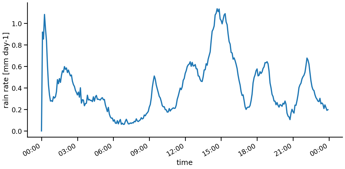
[16]:
fig = plt.figure( figsize = (14,6))

plt.gca().xaxis.set_major_formatter(myFmt)
rain_mean.plot( lw = 3 )
sns.despine()
Tasks
Use this notebook to explore the time series of other variables.
How do different cloud cover variables look like?
How does LWP evolve? (variable
tqc_dia)How does CAPE look like?