Plotting Precipitation Overview Maps

Here, we combine several aspects explored in the previous notebooks. We will

• read the ICON grid file

• read multiple ICON 2D data file and extract information on precipitation and

• finally combine all precipitation fields to a multi-panel plot

Load Python Libraries

%matplotlib inline

# system libs
import os, sys, glob

# array operators and netcdf datasets
import numpy as np
import xarray as xr
import datetime

# plotting
import pylab as plt
import seaborn as sns
sns.set_context('talk')

# drawing onto a map
import cartopy.crs as ccrs
import cartopy.feature as cfeature
import cartopy.io.shapereader as shpreader

As mentioned in the notebook 03-Plottting_Precipitation_as_Time_Series.ipynb, here we will import our tools module. The imported function convert_timevec will handle the time axis in the ICON data.

sys.path.append( '/work/bb1224/2023_MS-COURSE/tools/analysis' )
from tools import convert_timevec

Open Data with xarray

General Paths

exercise_path = '/work/bb1224/2023_MS-COURSE'
data_path = f'{exercise_path}/data'
icon_data_path = f'{data_path}/icon-lem'

This is the content of the data directory:

os.listdir(icon_data_path)

['grids-extpar', 'experiments', 'bc-init']

grid_name = 'lpz_r2'
grid_path = f'{icon_data_path}/grids-extpar/{grid_name}'

exp_name = 'icon_lam_1dom_lpz-base'
exp_path = f'{icon_data_path}/experiments/{exp_name}'

Grid File

grid1 = xr.open_dataset( f'{grid_path}/lpz_r2_dom01_DOM01.nc', chunks={} )
# grid1 = xr.open_dataset( f'{grid_path}/lpz_r2_dom02_DOM02.nc', chunks={} )

Data Files

Again, we use the xarrayfunction open_mfdataset to read in multiple ICON datasets. The data are not load into memory, but handled as pointers.

dset = xr.open_mfdataset( f'{exp_path}/2d_cloud_DOM01_ML_20210516T*Z.nc', chunks={'time':1}, combine='by_coords' )
# dset = xr.open_mfdataset( f'{exp_path}/2d_cloud_DOM02_ML_20210516T*.nc', chunks={'time':1}, combine='by_coords' )

dset['time'] = convert_timevec( dset.time.data )

dset

<xarray.Dataset>
Dimensions:        (time: 288, plev: 1, bnds: 2, plev_2: 1, plev_3: 1,
                    ncells: 10212)
Coordinates:
  * time           (time) datetime64[ns] 2021-05-16 ... 2021-05-16T23:55:00
  * plev           (plev) float64 0.0
  * plev_2         (plev_2) float64 400.0
  * plev_3         (plev_3) float64 800.0
Dimensions without coordinates: bnds, ncells
Data variables: (12/17)
    plev_bnds      (time, plev, bnds) float64 dask.array<chunksize=(12, 1, 2), meta=np.ndarray>
    plev_2_bnds    (time, plev_2, bnds) float64 dask.array<chunksize=(12, 1, 2), meta=np.ndarray>
    plev_3_bnds    (time, plev_3, bnds) float64 dask.array<chunksize=(12, 1, 2), meta=np.ndarray>
    tqv_dia        (time, ncells) float32 dask.array<chunksize=(1, 10212), meta=np.ndarray>
    tqc_dia        (time, ncells) float32 dask.array<chunksize=(1, 10212), meta=np.ndarray>
    tqi_dia        (time, ncells) float32 dask.array<chunksize=(1, 10212), meta=np.ndarray>
    ...             ...
    cape           (time, ncells) float32 dask.array<chunksize=(1, 10212), meta=np.ndarray>
    cape_ml        (time, ncells) float32 dask.array<chunksize=(1, 10212), meta=np.ndarray>
    cin_ml         (time, ncells) float32 dask.array<chunksize=(1, 10212), meta=np.ndarray>
    rain_con_rate  (time, ncells) float32 dask.array<chunksize=(1, 10212), meta=np.ndarray>
    prec_con       (time, ncells) float32 dask.array<chunksize=(1, 10212), meta=np.ndarray>
    prec_gsp       (time, ncells) float32 dask.array<chunksize=(1, 10212), meta=np.ndarray>
Attributes:
    CDI:                  Climate Data Interface version 1.8.4 (http://mpimet...
    Conventions:          CF-1.6
    number_of_grid_used:  99
    uuidOfHGrid:          718d4bb6-2c67-4c84-a5ab-440d28412a00
    institution:          Max Planck Institute for Meteorology/Deutscher Wett...
    title:                ICON simulation
    source:               @
    history:              /home/k/k206107/workspace/icon-build/bin/icon at 20...
    references:           see MPIM/DWD publications
    comment:              v107 Workshop (k206107) on l30004 (Linux 4.18.0-348...

xarray.Dataset

• Dimensions:
  • time: 288
  • plev: 1
  • bnds: 2
  • plev_2: 1
  • plev_3: 1
  • ncells: 10212
• Coordinates: (4)
  • time
    (time)
    datetime64[ns]
    2021-05-16 ... 2021-05-16T23:55:00

    array(['2021-05-16T00:00:00.000000000', '2021-05-16T00:05:00.000000000',
           '2021-05-16T00:10:00.000000000', ..., '2021-05-16T23:45:00.000000000',
           '2021-05-16T23:50:00.000000000', '2021-05-16T23:55:00.000000000'],
          dtype='datetime64[ns]')

  • plev
    (plev)
    float64
    0.0

    standard_name :

    air_pressure

    long_name :

    pressure

    units :

    hPa

    positive :

    down

    axis :

    Z

    bounds :

    plev_bnds

    array([0.])

  • plev_2
    (plev_2)
    float64
    400.0

    standard_name :

    air_pressure

    long_name :

    pressure

    units :

    hPa

    positive :

    down

    axis :

    Z

    bounds :

    plev_2_bnds

    array([400.])

  • plev_3
    (plev_3)
    float64
    800.0

    standard_name :

    air_pressure

    long_name :

    pressure

    units :

    hPa

    positive :

    down

    axis :

    Z

    bounds :

    plev_3_bnds

    array([800.])

• Data variables: (17)
  • plev_bnds
    (time, plev, bnds)
    float64
    dask.array<chunksize=(12, 1, 2), meta=np.ndarray>

    Array Chunk Bytes 4.50 kiB 192 B Shape (288, 1, 2) (12, 1, 2) Dask graph 24 chunks in 73 graph layers Data type float64 numpy.ndarray

  • plev_2_bnds
    (time, plev_2, bnds)
    float64
    dask.array<chunksize=(12, 1, 2), meta=np.ndarray>

    Array Chunk Bytes 4.50 kiB 192 B Shape (288, 1, 2) (12, 1, 2) Dask graph 24 chunks in 73 graph layers Data type float64 numpy.ndarray

  • plev_3_bnds
    (time, plev_3, bnds)
    float64
    dask.array<chunksize=(12, 1, 2), meta=np.ndarray>

    Array Chunk Bytes 4.50 kiB 192 B Shape (288, 1, 2) (12, 1, 2) Dask graph 24 chunks in 73 graph layers Data type float64 numpy.ndarray

  • tqv_dia
    (time, ncells)
    float32
    dask.array<chunksize=(1, 10212), meta=np.ndarray>

    standard_name :

    tqv_dia

    long_name :

    total column integrated water vapour (diagnostic)

    units :

    kg m**-2

    param :

    214.1.0

    CDI_grid_type :

    unstructured

    number_of_grid_in_reference :

    1

    Array Chunk Bytes 11.22 MiB 39.89 kiB Shape (288, 10212) (1, 10212) Dask graph 288 chunks in 49 graph layers Data type float32 numpy.ndarray

  • tqc_dia
    (time, ncells)
    float32
    dask.array<chunksize=(1, 10212), meta=np.ndarray>

    standard_name :

    tqc_dia

    long_name :

    total column integrated cloud water (diagnostic)

    units :

    kg m**-2

    param :

    215.1.0

    CDI_grid_type :

    unstructured

    number_of_grid_in_reference :

    1

    Array Chunk Bytes 11.22 MiB 39.89 kiB Shape (288, 10212) (1, 10212) Dask graph 288 chunks in 49 graph layers Data type float32 numpy.ndarray

  • tqi_dia
    (time, ncells)
    float32
    dask.array<chunksize=(1, 10212), meta=np.ndarray>

    standard_name :

    tqi_dia

    long_name :

    total column integrated cloud ice (diagnostic)

    units :

    kg m**-2

    param :

    216.1.0

    CDI_grid_type :

    unstructured

    number_of_grid_in_reference :

    1

    Array Chunk Bytes 11.22 MiB 39.89 kiB Shape (288, 10212) (1, 10212) Dask graph 288 chunks in 49 graph layers Data type float32 numpy.ndarray

  • clct
    (time, ncells)
    float32
    dask.array<chunksize=(1, 10212), meta=np.ndarray>

    standard_name :

    clct

    long_name :

    total cloud cover

    units :

    %

    param :

    1.6.0

    CDI_grid_type :

    unstructured

    number_of_grid_in_reference :

    1

    Array Chunk Bytes 11.22 MiB 39.89 kiB Shape (288, 10212) (1, 10212) Dask graph 288 chunks in 49 graph layers Data type float32 numpy.ndarray

  • rain_gsp_rate
    (time, ncells)
    float32
    dask.array<chunksize=(1, 10212), meta=np.ndarray>

    standard_name :

    rain_gsp_rate

    long_name :

    gridscale rain rate

    units :

    kg m-2 s-1

    param :

    77.1.0

    CDI_grid_type :

    unstructured

    number_of_grid_in_reference :

    1

    Array Chunk Bytes 11.22 MiB 39.89 kiB Shape (288, 10212) (1, 10212) Dask graph 288 chunks in 49 graph layers Data type float32 numpy.ndarray

  • clch
    (time, plev, ncells)
    float32
    dask.array<chunksize=(1, 1, 10212), meta=np.ndarray>

    standard_name :

    clch

    long_name :

    high level clouds

    units :

    %

    param :

    22.6.0

    CDI_grid_type :

    unstructured

    number_of_grid_in_reference :

    1

    Array Chunk Bytes 11.22 MiB 39.89 kiB Shape (288, 1, 10212) (1, 1, 10212) Dask graph 288 chunks in 49 graph layers Data type float32 numpy.ndarray

  • clcm
    (time, plev_2, ncells)
    float32
    dask.array<chunksize=(1, 1, 10212), meta=np.ndarray>

    standard_name :

    clcm

    long_name :

    mid level clouds

    units :

    %

    param :

    22.6.0

    CDI_grid_type :

    unstructured

    number_of_grid_in_reference :

    1

    Array Chunk Bytes 11.22 MiB 39.89 kiB Shape (288, 1, 10212) (1, 1, 10212) Dask graph 288 chunks in 49 graph layers Data type float32 numpy.ndarray

  • clcl
    (time, plev_3, ncells)
    float32
    dask.array<chunksize=(1, 1, 10212), meta=np.ndarray>

    standard_name :

    clcl

    long_name :

    low level clouds

    units :

    %

    param :

    22.6.0

    CDI_grid_type :

    unstructured

    number_of_grid_in_reference :

    1

    Array Chunk Bytes 11.22 MiB 39.89 kiB Shape (288, 1, 10212) (1, 1, 10212) Dask graph 288 chunks in 49 graph layers Data type float32 numpy.ndarray

  • cape
    (time, ncells)
    float32
    dask.array<chunksize=(1, 10212), meta=np.ndarray>

    standard_name :

    cape

    long_name :

    conv avail pot energy

    units :

    J kg-1

    param :

    6.7.0

    CDI_grid_type :

    unstructured

    number_of_grid_in_reference :

    1

    Array Chunk Bytes 11.22 MiB 39.89 kiB Shape (288, 10212) (1, 10212) Dask graph 288 chunks in 49 graph layers Data type float32 numpy.ndarray

  • cape_ml
    (time, ncells)
    float32
    dask.array<chunksize=(1, 10212), meta=np.ndarray>

    standard_name :

    cape_ml

    long_name :

    cape of mean surface layer parcel

    units :

    J kg-1

    param :

    6.7.0

    CDI_grid_type :

    unstructured

    number_of_grid_in_reference :

    1

    Array Chunk Bytes 11.22 MiB 39.89 kiB Shape (288, 10212) (1, 10212) Dask graph 288 chunks in 49 graph layers Data type float32 numpy.ndarray

  • cin_ml
    (time, ncells)
    float32
    dask.array<chunksize=(1, 10212), meta=np.ndarray>

    standard_name :

    cin_ml

    long_name :

    convective inhibition of mean surface layer parcel

    units :

    J kg-1

    param :

    7.7.0

    CDI_grid_type :

    unstructured

    number_of_grid_in_reference :

    1

    Array Chunk Bytes 11.22 MiB 39.89 kiB Shape (288, 10212) (1, 10212) Dask graph 288 chunks in 49 graph layers Data type float32 numpy.ndarray

  • rain_con_rate
    (time, ncells)
    float32
    dask.array<chunksize=(1, 10212), meta=np.ndarray>

    standard_name :

    rain_con_rate

    long_name :

    convective rain rate

    units :

    kg m-2 s-1

    param :

    76.1.0

    CDI_grid_type :

    unstructured

    number_of_grid_in_reference :

    1

    Array Chunk Bytes 11.22 MiB 39.89 kiB Shape (288, 10212) (1, 10212) Dask graph 288 chunks in 49 graph layers Data type float32 numpy.ndarray

  • prec_con
    (time, ncells)
    float32
    dask.array<chunksize=(1, 10212), meta=np.ndarray>

    standard_name :

    prec_con

    long_name :

    convective precip

    units :

    kg m-2

    param :

    37.1.0

    CDI_grid_type :

    unstructured

    number_of_grid_in_reference :

    1

    Array Chunk Bytes 11.22 MiB 39.89 kiB Shape (288, 10212) (1, 10212) Dask graph 288 chunks in 49 graph layers Data type float32 numpy.ndarray

  • prec_gsp
    (time, ncells)
    float32
    dask.array<chunksize=(1, 10212), meta=np.ndarray>

    standard_name :

    prec_gsp

    long_name :

    gridscale precip

    units :

    kg m-2

    param :

    54.1.0

    CDI_grid_type :

    unstructured

    number_of_grid_in_reference :

    1

    Array Chunk Bytes 11.22 MiB 39.89 kiB Shape (288, 10212) (1, 10212) Dask graph 288 chunks in 49 graph layers Data type float32 numpy.ndarray

• Indexes: (4)
  • time
    PandasIndex

    PandasIndex(DatetimeIndex(['2021-05-16 00:00:00', '2021-05-16 00:05:00',
                   '2021-05-16 00:10:00', '2021-05-16 00:15:00',
                   '2021-05-16 00:20:00', '2021-05-16 00:25:00',
                   '2021-05-16 00:30:00', '2021-05-16 00:35:00',
                   '2021-05-16 00:40:00', '2021-05-16 00:45:00',
                   ...
                   '2021-05-16 23:10:00', '2021-05-16 23:15:00',
                   '2021-05-16 23:20:00', '2021-05-16 23:25:00',
                   '2021-05-16 23:30:00', '2021-05-16 23:35:00',
                   '2021-05-16 23:40:00', '2021-05-16 23:45:00',
                   '2021-05-16 23:50:00', '2021-05-16 23:55:00'],
                  dtype='datetime64[ns]', name='time', length=288, freq=None))

  • plev
    PandasIndex

    PandasIndex(Index([0.0], dtype='float64', name='plev'))

  • plev_2
    PandasIndex

    PandasIndex(Index([400.0], dtype='float64', name='plev_2'))

  • plev_3
    PandasIndex

    PandasIndex(Index([800.0], dtype='float64', name='plev_3'))

• Attributes: (10)

  CDI :

  Climate Data Interface version 1.8.4 (http://mpimet.mpg.de/cdi)

  Conventions :

  CF-1.6

  number_of_grid_used :

  99

  uuidOfHGrid :

  718d4bb6-2c67-4c84-a5ab-440d28412a00

  institution :

  Max Planck Institute for Meteorology/Deutscher Wetterdienst

  title :

  ICON simulation

  source :

  @

  history :

  /home/k/k206107/workspace/icon-build/bin/icon at 20230531 080330

  references :

  see MPIM/DWD publications

  comment :

  v107 Workshop (k206107) on l30004 (Linux 4.18.0-348.el8.x86_64 x86_64)

Prepare Precip Data

Again, we need to combine grid-scale and subgrid-scale contributions to precipitation.

• Do you understand why we have two parts?

• Which model parameterization is responsible for which part?

rain = dset['rain_con_rate'] + dset['rain_gsp_rate']
rain.attrs['long_name'] = 'rain rate'

conversion_factor = 3600 * 24

rain = conversion_factor * rain
rain.attrs['units'] = 'mm day-1'

rain

<xarray.DataArray (time: 288, ncells: 10212)>
dask.array<mul, shape=(288, 10212), dtype=float64, chunksize=(1, 10212), chunktype=numpy.ndarray>
Coordinates:
  * time     (time) datetime64[ns] 2021-05-16 ... 2021-05-16T23:55:00
Dimensions without coordinates: ncells
Attributes:
    units:    mm day-1

xarray.DataArray

• time: 288
• ncells: 10212

• dask.array<chunksize=(1, 10212), meta=np.ndarray>

  Array Chunk Bytes 22.44 MiB 79.78 kiB Shape (288, 10212) (1, 10212) Dask graph 288 chunks in 100 graph layers Data type float64 numpy.ndarray

• Coordinates: (1)
  • time
    (time)
    datetime64[ns]
    2021-05-16 ... 2021-05-16T23:55:00

    array(['2021-05-16T00:00:00.000000000', '2021-05-16T00:05:00.000000000',
           '2021-05-16T00:10:00.000000000', ..., '2021-05-16T23:45:00.000000000',
           '2021-05-16T23:50:00.000000000', '2021-05-16T23:55:00.000000000'],
          dtype='datetime64[ns]')

• Indexes: (1)
  • time
    PandasIndex

    PandasIndex(DatetimeIndex(['2021-05-16 00:00:00', '2021-05-16 00:05:00',
                   '2021-05-16 00:10:00', '2021-05-16 00:15:00',
                   '2021-05-16 00:20:00', '2021-05-16 00:25:00',
                   '2021-05-16 00:30:00', '2021-05-16 00:35:00',
                   '2021-05-16 00:40:00', '2021-05-16 00:45:00',
                   ...
                   '2021-05-16 23:10:00', '2021-05-16 23:15:00',
                   '2021-05-16 23:20:00', '2021-05-16 23:25:00',
                   '2021-05-16 23:30:00', '2021-05-16 23:35:00',
                   '2021-05-16 23:40:00', '2021-05-16 23:45:00',
                   '2021-05-16 23:50:00', '2021-05-16 23:55:00'],
                  dtype='datetime64[ns]', name='time', length=288, freq=None))

• Attributes: (1)

  units :

  mm day-1

Plotting Precip Maps

Shortcuts for Fieldnames

# read center lon/lat in radiant
clon_rad = grid1['clon']                # center longitude  / rad
clat_rad = grid1['clat']                # center latitutde  / rad

# convert to degrees
clon = np.rad2deg( clon_rad )
clat = np.rad2deg( clat_rad )

# select a subset, each 12th time slot
rr  = rain.isel( time = slice(0, None, 12) )

Plotting Precip onto a Map

The map plotting is borrowed from the notebook 01-Plotting-ICON-Topography.ipynb.

Define States

# read shape file
shape_file = f'{data_path}/shapes/vg2500_bld.shp'
reader = shpreader.Reader( shape_file )

#  and create cartopy feature
states_data = list(reader.geometries())
states = cfeature.ShapelyFeature(states_data, ccrs.PlateCarree())

Make a Multi-Panel Plot

fig = plt.figure( figsize = (20,20) )
plt.subplots_adjust( wspace = 0.05, hspace = 0.1) # it looks nicer if spaces between subpanels are smaller

rr_values = [0, 0.1, 0.5, 1, 2, 5, 8, 10, 15, 20, 30, 50]
norm = plt.matplotlib.colors.BoundaryNorm(boundaries = rr_values, ncolors = 256, )

for i in range( 24 ):

    ax = plt.subplot(6,4,i+1, projection = ccrs.PlateCarree() )
    ax.add_feature(cfeature.LAND, facecolor='lightgray')

    v =  rr.isel( time = i )
    plt.tricontourf( clon, clat, v,
                     levels = rr_values,
                     cmap = plt.cm.CMRmap_r,
                     norm = norm,
                     extend = 'both'
                   )
    # and here we draw country borders
    ax.add_feature(cfeature.BORDERS.with_scale('50m'), linewidth = 2)
    ax.add_feature(states, facecolor='none', edgecolor='black', linewidth = 0.4)

    # write time as string in the corner
    t = v.time.data.astype('datetime64[m]')
    date, time  = str( t ).split('T')
    ax.text( 14.8, 53.3, time[:5])

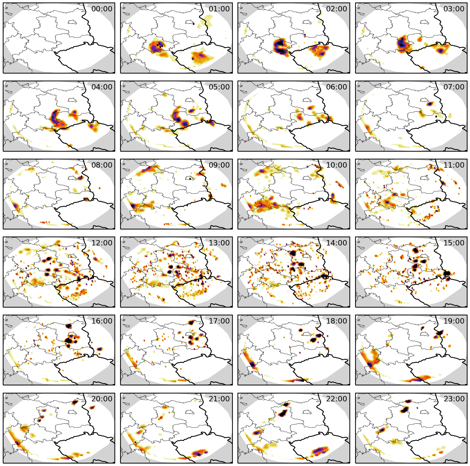
How do the plots look like if you choose a different matplotlib colormap (see here: https://matplotlib.org/stable/tutorials/colors/colormaps.html )?

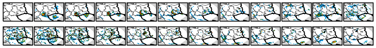
A “nice” Colormap from blue to red

cmap_new =  plt.matplotlib.colors.LinearSegmentedColormap.from_list('rr_colors',
                                        ['white', '#1ca8e9','#097cc4', '#095389',
                                         'forestgreen','yellowgreen',  'gold','orangered',
                                         'brown', 'black'], gamma = 1.)

fig = plt.figure( figsize = (16,2) )
plt.subplots_adjust( wspace = 0.05, hspace = 0.1) # it looks nicer if spaces between subpanels are smaller

rr_values = [0, 0.1, 0.5, 1, 2, 5, 8, 10, 15, 20, 30, 50]
norm = plt.matplotlib.colors.BoundaryNorm(boundaries = rr_values, ncolors = 256, )

for i in range( 24 ):

    ax = plt.subplot(2,12,i+1, projection = ccrs.PlateCarree() )
    ax.add_feature(cfeature.LAND, facecolor='lightgray')


    plt.tricontourf( clon, clat, rr.isel( time = i ),
                     levels = rr_values,
                     cmap = cmap_new,
                     extend = 'both',
                     norm = norm
                    )


    # and here we draw country borders
    ax.add_feature(cfeature.BORDERS.with_scale('50m'), linewidth = 2)
    ax.add_feature(states, facecolor='none', edgecolor='black', linewidth = 0.4)

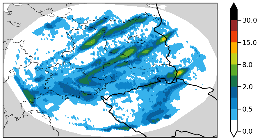
Accumulated Rain

Calculating the rain accumulation is easy! We already have rain in mm day-1 and the output frequency is regular. So, we just take the average a get the average rain in mm day-1.

fig = plt.figure( figsize = (12,6) )
plt.subplots_adjust( wspace = 0.05, hspace = 0.1) # it looks nicer if spaces between subpanels are smaller

rr_values = [0, 0.1, 0.5, 1, 2, 5, 8, 10, 15, 20, 30, 50]
norm = plt.matplotlib.colors.BoundaryNorm(boundaries = rr_values, ncolors = 256, )

rain_accu = rain.mean('time').compute()

ax = plt.subplot(1,1,1, projection = ccrs.PlateCarree() )
ax.add_feature(cfeature.LAND, facecolor='lightgray')


plt.tricontourf( clon, clat, rain_accu,
                     levels = rr_values,
                     cmap = cmap_new,
                     extend = 'both',
                     norm = norm
                    )
plt.colorbar()

# and here we draw country borders
ax.add_feature(cfeature.BORDERS.with_scale('50m'), linewidth = 2)
ax.add_feature(states, facecolor='none', edgecolor='black', linewidth = 0.4)

<cartopy.mpl.feature_artist.FeatureArtist at 0x7fff8f5a2800>

Tasks

Please explore the data with this notebook:

• Check how the temporal evolution looks like for

  • total cloud cover, variable name clct

  • liquid water path, variable name: tqc_dia

  • ice water path, variable name: tqi_dia